
We'll show you 5 different methods
When you want to compare values in different columns in Microsoft Excel, you can use more than just your eyeballs. You can highlight unique or duplicate values, display True or False for matches, or see which exact values appear in both columns.
We’ll show you how to compare two columns in Excel using five different methods. This lets you choose the one that best fits your needs and the data in your Excel worksheet.
Table of Contents
Highlight Unique or Duplicate Values With Conditional Formatting
If you want to spot the duplicates or the unique values in your columns, you can set up a conditional formatting rule. Once you see the values highlighted, you can take whatever action you need.
Using this method, the rule compares the values in the columns overall, not per row.
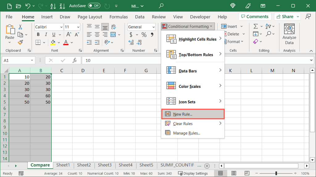
- Select the columns you want to compare. Then, go to the Home tab, open the Conditional Formatting drop-down menu, and choose New Rule.
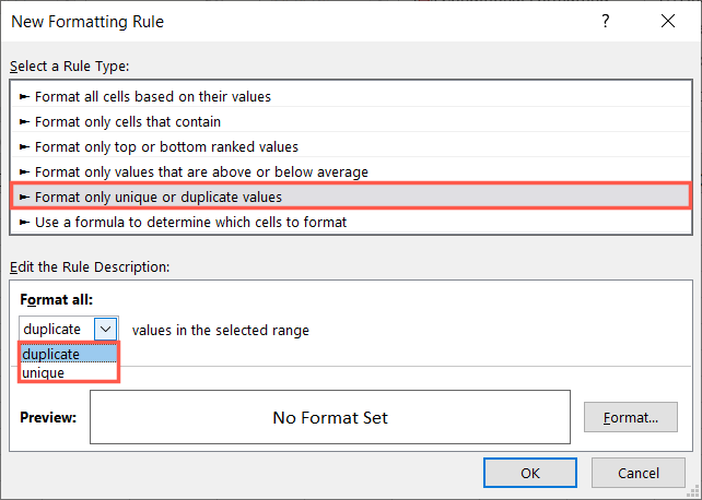
- Pick Format only unique or duplicate values at the top of the New Formatting Rule box.
- In the Format all drop-down box, choose either unique or duplicate, depending on which you prefer to highlight.
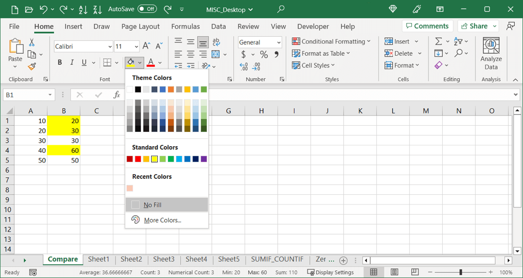
- Select the Format button and use the tabs to choose the formatting style you want. For instance, you can use the Font tab to pick a color for the text or the Fill tab to pick a color for the cells. Select OK.

- You’ll then see a preview of how your unique or duplicate values will appear. Select OK to apply the rule.

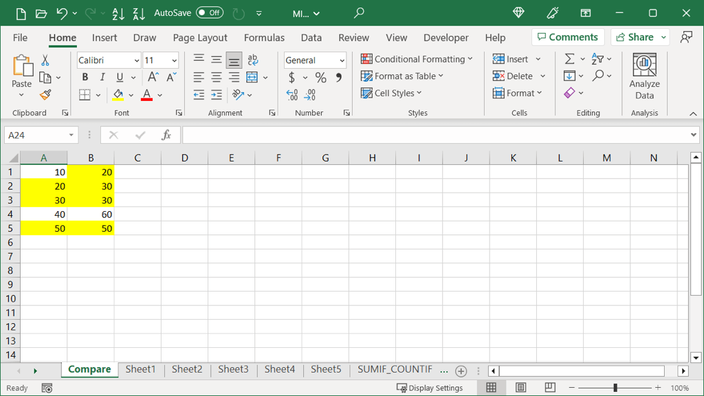
When you see the values highlighted, you can take action on them as you please. In this example, we’ve filled the cells with duplicate values yellow.
Compare Columns Using Go To Special
If you want to see the differences in your columns by row, you can use the Go To Special feature. This temporarily highlights the unique values so that you can do what you need.
Remember, using this method, the feature compares the values per row, not overall.
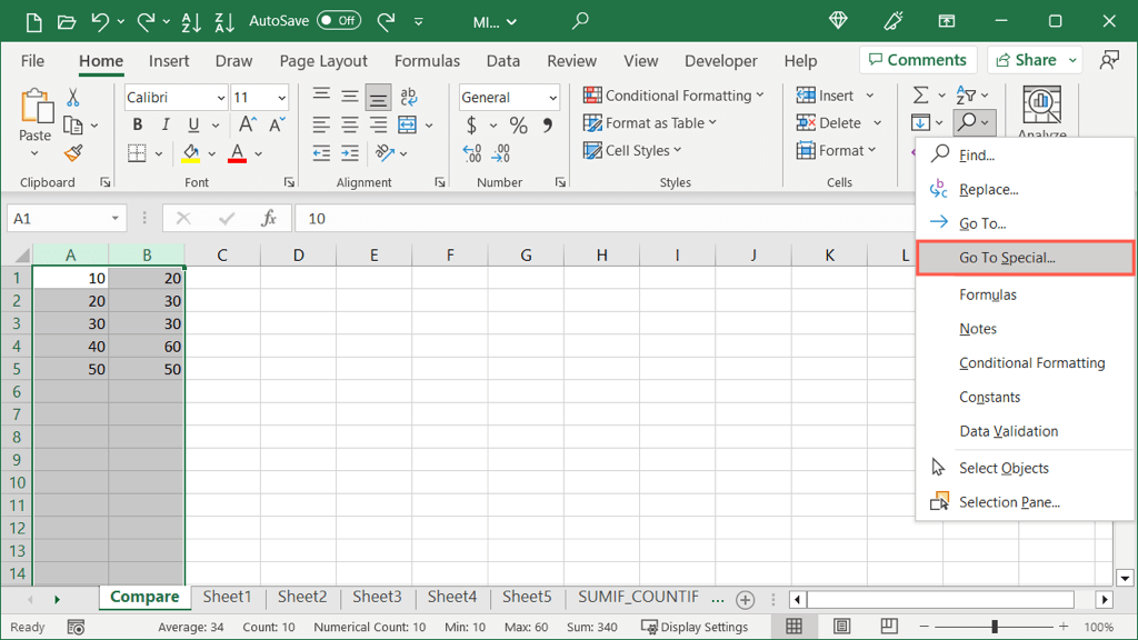
- Select the columns or cells in the columns you want to compare. Go to the Home tab, open the Find & Select drop-down menu, and choose Go To Special.
- In the dialog box that appears, pick Row differences and select OK.

- You’ll then see cells in the rows selected in the second column that are different from the first.

You can take action immediately if you only have a few differences. If you have many, you can keep the cells selected and choose a Fill Color on the Home tab to permanently highlight the cells. This gives you more time to do what you need.
Compare Columns Using True or False
Maybe you prefer to find matches and differences in your dataset without font or cell formatting. You can use a simple formula without a function to display True for values that are the same or False for those that are not.
Using this method, the formula compares the values per row, not overall.
- Go to the row containing the first two values you want to compare and select the cell to the right.
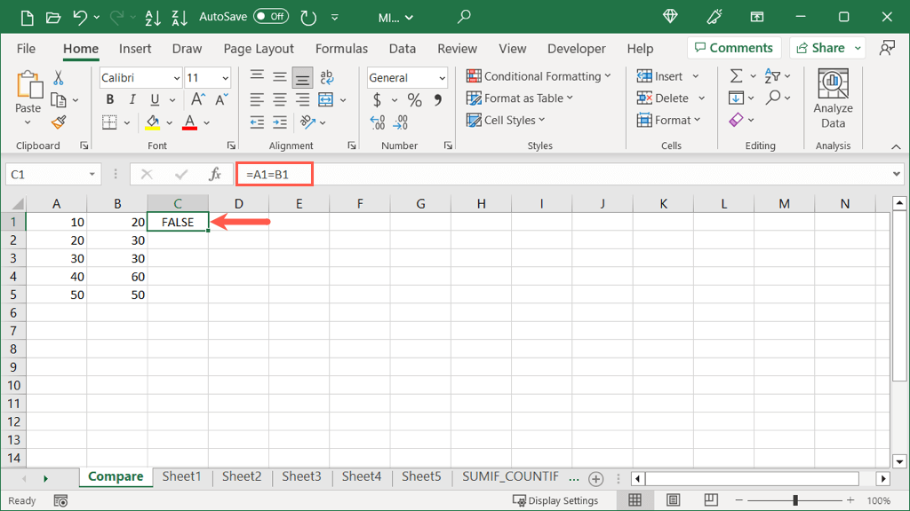
- Type an equal sign (=), the first cell reference, another equal sign, and the second cell reference. Then, press Enter or Return to see the result. As an example, we’ll compare cells A1 and B1 using the following formula:
=A1=B1

- You can then use the fill handle to copy and paste that formula to the remaining cells in the columns. Either drag the fill handle downward to fill the cells or double-click it to automatically fill the rest of the cells.

You’ll then have a True or False in that column for each row of values.
Compare Columns Using the IF Function
If you like the above method for showing a simple True or False for your values, but prefer to display something different, you can use the IF function. With it, you can enter the text you want to show for duplicate and unique values.
Like the above example, the formula compares the values per row, not overall.
The syntax for the formula is IF(test, if_true, if_false).
- Test: Enter the values you want to compare. For finding unique or duplicate values, you’ll use the cell references with an equal sign between them (shown below).
- If_true: Enter the text or value to display if the values match. Place this within quotation marks.
- If_false: Enter the text or value to display if the values don’t match. Place this in quotes as well.
Go to the row containing the first two values you want to compare and select the cell to the right as shown earlier.
Then, enter the IF function and its formula. Here, we’ll compare cells A1 and B1. If they are the same, we’ll display “Same” and if they’re not, we’ll display “Different.”
=IF(A1=B1,”Same”,”Different”)
Once you receive the result, you can use the fill handle as described earlier to fill the remaining cells in the column to see the rest of the results.

Compare Columns Using the VLOOKUP Function
One more way to compare columns in Excel is using the VLOOKUP function. With its formula, you can see which values are the same in both columns.
The syntax for the formula is VLOOKUP(lookup_value, array, col_num, match).
- Lookup_value: The value you want to look up. You’ll start with the cell on the left of that row and then copy the formula down for the remaining cells.
- Array: The range of cells to look up the above value.
- Col_num: The column number that contains the return value.
- Match: Enter 1 or True for an approximate match or 0 or False for an exact match.
Go to the row containing the first two values you want to compare and select the cell to the right as shown earlier.
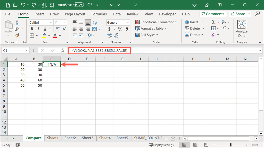
Then, enter the VLOOKUP function and its formula. Here, we’ll start with cell A1 in the first column for an exact match.
=VLOOKUP(A1,$B$1:$B$5,1,FALSE)

Notice that we use absolute references ($B$1:$B$5) rather than relative references (B1:B5). This is so we can copy the formula down to the remaining cells while keeping the same range in the array argument.
Select the fill handle and drag to the remaining cells or double-click to fill them.
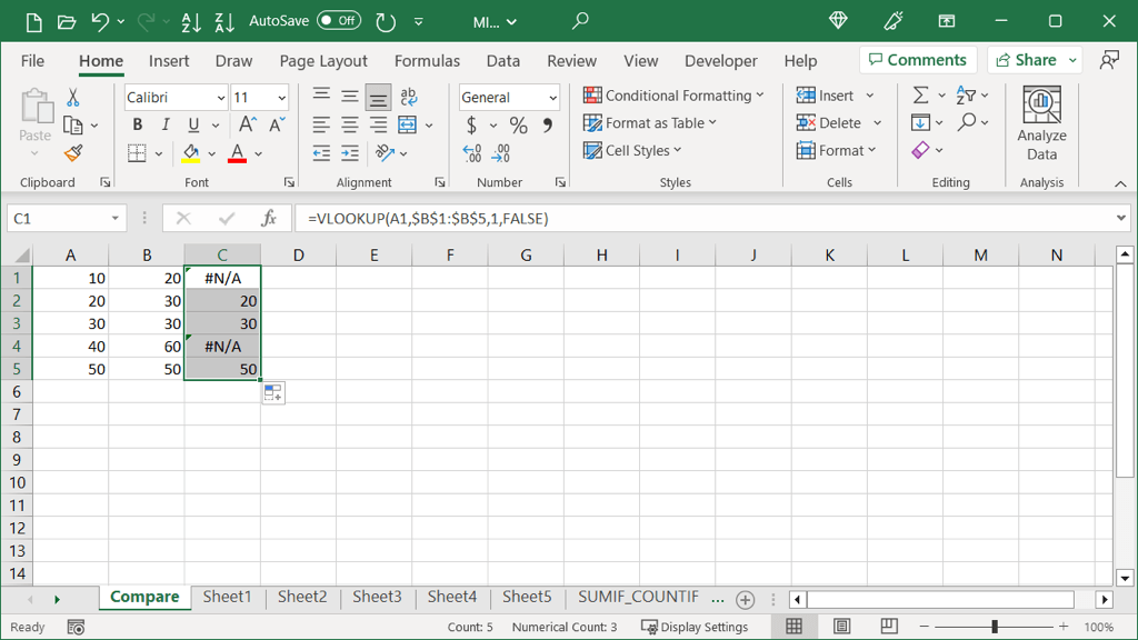
You can see that the formula returns results for those values in column B that also appear in column A. For those values that do not, you’ll see the #N/A error.

Optional: Add the IFNA Function
If you prefer to display something other than #N/A for non-matching data, you can add the IFNA function to the formula.
The syntax is IFNA(value, if_na) where the value is where you’re checking for the #N/A and if_na is what to display if it’s found.
Here, we’ll display an asterisk instead of #N/A using this formula:
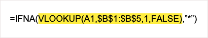
=IFNA(VLOOKUP(A1,$B$1:$B$5,1,FALSE),”*”)
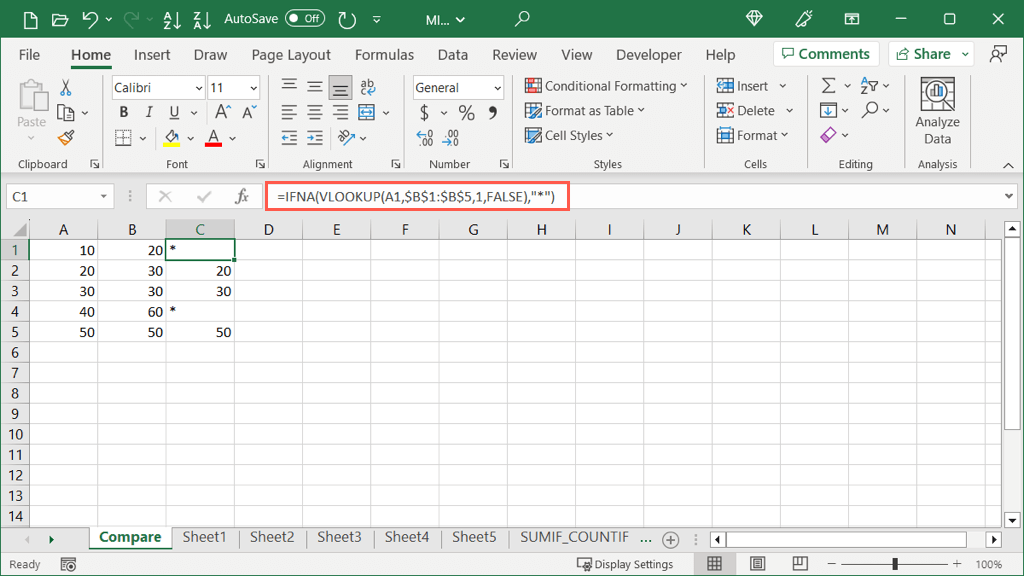
As you can see, we simply insert the VLOOKUP formula as the first argument for the IFNA formula. Then we add the second argument, which is the asterisk in quotes at the end. You can also insert a space or other character within quotes if you prefer.
Using built-in features or Excel formulas, you can compare spreadsheet data in a variety of ways. Whether for data analysis or simply spotting matching values, you can use one or all of these methods in Excel.
Subscribe on YouTube!
Did you enjoy this tip? If so, check out our YouTube channel from our sister site Online Tech Tips. We cover Windows, Mac, software and apps, and have a bunch of troubleshooting tips and how-to videos. Click the button below to subscribe!
Subscribe